Disclaimer: This tutorial is primarily based on a knowledge-sharing session I conducted at work. While the session provided the inspiration and foundation for the content, all examples, explanations, code, and opinions presented here are my own and are intended solely for educational purposes. Nothing in this tutorial represents, reflects, or should be interpreted as the views, practices, or intellectual property of my employer.

Modern language models can appear remarkably intelligent, but at their core they perform a deceptively simple operation:

Given the text so far, predict the next word.

While the objective sounds very simple, achiving it requires a surprisingly sophisticated pipeline.

Before a model can predict the next token, it needs to:

1. convert text into discrete token IDs,
2. represent those tokens as vectors,
3. incorporate information from surrounding context,
4. determine which parts of that context are relevant,
5. produce a probability distribution over the vocabulary,
6. and finally select the next token.

This tutorial follows that journey from raw text to token IDs, from token IDs to embeddings, from embeddings to contextual representations, and finally to self-attention and real attention maps.

The goal is not merely to learn the terminology. By the end, you should have a mental model for what happens inside a Transformer when it processes a sentence.

⋅ • ✦ • ⋅

The Big Picture

A simplified language-model pipeline looks like the following

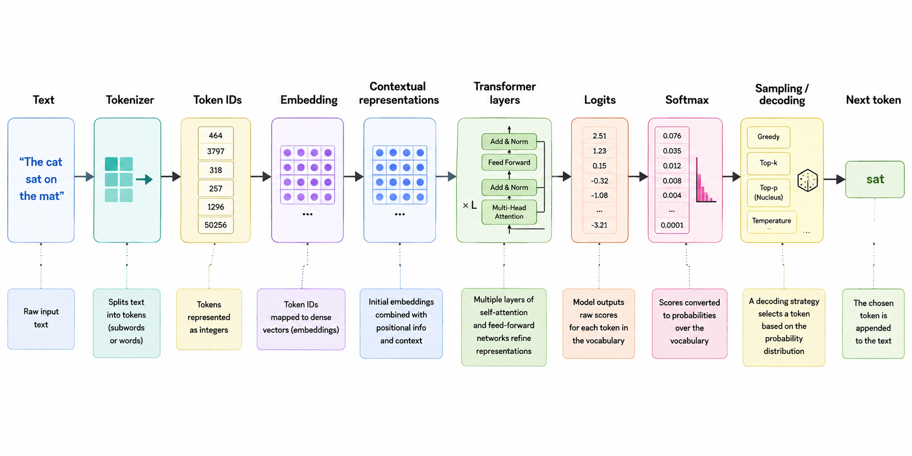
Each stage solves a different problem.

Tokenization converts language into a discrete representation that a neural network can process. Tokens can be words, subwords, or even characters.

Embeddings convert discrete token IDs into continuous vectors. We dont want to feed raw integers into a neural network, neither do we want to use one-hot vectors. Instead, we learn a dense vector representation for each token.

Contextual representations allow each token to incorporate information from surrounding tokens and also it’s own position. A token’s representation is no longer static; it changes depending on the context in which it appears.

Self-attention allows each token to dynamically incorporate information from other tokens.

Logits represent the model’s raw preference for every possible next token.

Softmax converts those scores into probabilities.

Sampling or decoding determines which token is actually selected.

Understanding this pipeline provides a foundation for understanding modern large language models.

⋅ • ✦ • ⋅

Tokenization: Turning Text into Numbers

Neural networks do not directly operate on strings. They operate on numerical tensors.

The first step is therefore to convert text into a sequence of token IDs. This is the job of the tokenizer. In simple terms, a tokenizer maps text to a sequence of discrete integers, where each integer represents a token. The total number of unique tokens that can be represented by these IDs is called the vocabulary size. While the exact vocabulary size is not publicly disclosed for proprietary models, it is generally understood that models such as GPT-4o use a vocabulary of roughly 200,000 tokens.

Tokenizers do not necessarily map text directly to whole words. A token can represent a word, subword, or even a single character or byte, depending on the tokenizer. Modern GPT-style models commonly use subword tokenization techniques such as Byte Pair Encoding (BPE). Rather than creating a vocabulary entry for every possible word, BPE builds its vocabulary from frequently occurring sequences of characters or bytes, allowing it to represent both common words and previously unseen words efficiently.

BPE is a subword segmentation algorithm that iteratively merges the most frequent pairs of bytes or characters in a text corpus. This approach allows the tokenizer to efficiently handle rare and unknown words by breaking them into smaller, more common subword units. BPE is widely used in modern NLP models because it balances vocabulary size and coverage, enabling robust tokenization for diverse languages and domains.

⋅ • ✦ • ⋅

Why not simply tokenize by word?

Suppose we used a word-level tokenizer to tokenize the sentence:

I am going to do some model architecting

A sentence might become:

I → 1
am → 2
going → 3
to → 4
do → 5
some → 6
model → 7
architecting → 8

This seems straightforward, but natural language contains an enormous number of words, names, misspellings, technical terms, abbreviations, and newly created words. A word-level vocabulary would either become enormous or encounter many unknown words.

Subword tokenization addresses this problem by allowing words to be represented as combinations of smaller pieces. For example, a word such as:

architecting

might be represented using:

architect + ing

This mean now we don’t need to have the word ‘architecting’ and ‘architect’ in the vocabulary. Instead, we can represent ‘architecting’ as a combination of two known subwords. This will also allow the model to represent previously unseen words as combinations of known subwords.

⋅ • ✦ • ⋅

Tokenization Defines the Model’s Modeling Space

It is tempting to think of tokenization as merely a preprocessing step. It has much more fundamental implications than that. My view is that the tokenization is where we need our research focus to be, because it defines the discrete space in which the model operates.

If a model has a vocabulary containing 200k tokens, its output layer ultimately needs to produce a score for approximately 200,000 possible next tokens.

That means the tokenizer affects:

• sequence length,
• vocabulary size,
• memory requirements,
• computational cost,
• how efficiently language is represented,
• and how easily unusual words can be represented.

In other words:

Tokenization is part of the model architecture, not merely a preprocessing step, and it can affect the complexity of the entire model pipeline

⋅ • ✦ • ⋅

Text to Token IDs

Let’s see this in practice using the GPT-2 tokenizer.

Funfact: the word Pissu is a Sri Lankan mild slang word that means “crazy”. I wanted to use something that would most likely be broken down into multiple subwords

import tiktoken

tokenizer = tiktoken.get_encoding("gpt2")
text = "I am going to do some model architecting by Googling, Pissu"
tokens = tokenizer.encode(text, allowed_special={"<|endoftext|>"})
print('tokens:', tokens)
print('num tokens:', len(tokens))

## Output
tokens: [40, 716, 1016, 284, 466, 617, 2746, 7068, 278, 416, 1514, 519, 1359, 11, 350, 747, 84]
num tokens: 17

The sentence has been converted into 17 token IDs.

These integers however, are not semantic values in themselves. For example, token ID 40 is not “more meaningful” than token ID 716. The IDs are simply indexes into the tokenizer’s vocabulary.

We can inspect what each token represents:

[f"{tid} -> {tokenizer.decode([tid])}" for tid in tokens]

### Output
['40-I',
 '716- am',
 '1016- going',
 '284- to',
 '466- do',
 '617- some',
 '2746- model',
 '7068- architect',
 '278-ing',
 '416- by',
 '1514- Go',
 '519-og',
 '1359-ling',
 '11-,',
 '350- P',
 '747-iss',
 '84-u']

This output illustrates an important property of modern tokenization.

Tokens are not necessarily words.

For example, ‘architecting’ has been split into ‘architect’ and ‘ing’. Similarly, ‘Googling’ has been split into ‘Go’, ‘og’, and ’ling’. Even the slang word ‘Pissu’, which is definetely is not a commonly encoutered word, has been split into ‘P’, ‘iss’, and ‘u’.

This is one of the reasons subword tokenization is so powerful, the model does not need a dedicated vocabulary entry for every possible word.

We can inspect the size of the GPT-2 tokenizer vocabulary that we have used above

tokenizer.n_vocab

## Output
50257

The vocabulary contains 50,257 token IDs, and 17 of these token IDs were used to represent the above sentence.

⋅ • ✦ • ⋅

From Token IDs to Probabilities

At this point we have converted language into numbers.

But there is still an important question:

How does a language model decide which token should come next?

Suppose the model receives:

"The capital of Australia is"

It might assign high scores to:

Canberra
Sydney
Melbourne
...

The model’s immediate output is not probabilities. It produces logits. A logit is an unnormalised score representing the model’s preference for a particular token.

For a vocabulary of size N, the model produces a vector of N logits, one for each token in the vocabulary. These values can be positive or negative and do not need to sum to anything in particular.

⋅ • ✦ • ⋅

Softmax: From Logits to Probabilities

To convert logits into a probability distribution, we use the softmax function:

$$ \text{softmax}(x_i) = \frac{e^{x_i}}{\sum_{j=1}^{N} e^{x_j}} $$

where N is the vocabulary size.

Softmax has two important properties:

1. Larger logits produce larger probabilities.
2. All probabilities sum to 1.

For example, conceptually, a model might produce:

Canberra    → 8.2
Sydney      → 5.1
Melbourne   → 4.7
banana      → -2.3
...

After softmax, those become probabilities between 0 and 1.

Canberra    → 0.99
Sydney      → 0.8
Melbourne   → 0.7
banana      → 0.001
...

The exact numbers are not important here. What matters is the transformation. This probability distribution represents the model’s uncertainty about what comes next.

⋅ • ✦ • ⋅

Choosing the Next Token

Once we have probabilities, we still need to choose a token.

There are several ways to do this.

Greedy Decoding

The simplest approach is to always choose the token with the highest probability. In the above example, the model will choose Canberra

This is predictable, but it can also produce repetitive or overly conservative text.

Temperature

Temperature adjust the logits before softmax transformation.

$$ \text{softmax}\left(\frac{x_i}{T}\right) $$

Temperature controls how concentrated the probability distribution becomes. Higher temperatures reduces the probability, producing flatter distributions, while lower temperatures produce sharper distributions.

For example for the above logits, if we choose higher T, Canberra’s probability might drop to 0.7, while Sydney and Melbourne’s probabilities increase to 0.5 and 0.4 respectively. Sampling from this distribution, will allow the model to explore less likely options.

⋅ • ✦ • ⋅

Top-k Sampling

The main disadvantage of converting all logits into probabilities using softmax is the computational cost. For every token generated, the model produces one logit for every token in its vocabulary. If the vocabulary contains 200,000 tokens, the model produces 200,000 logits, and softmax needs to process all of them to produce a probability distribution. This becomes increasingly expensive as vocabulary sizes grow, particularly because we only need to choose the next token, not calculate probabilities for every possible token with equal precision. One way to reduce this search space is top-k sampling. Instead of considering the entire vocabulary, top-k sampling keeps only the k tokens with the highest logits (and therefore the highest probabilities after softmax). All other tokens are discarded from consideration, and the model samples the next token only from this smaller set. For example, if:

k = 5

the model keeps the five most probable candidates and removes the rest before renormalising the probabilities.

This prevents extremely unlikely tokens from being selected while still allowing some randomness.

⋅ • ✦ • ⋅

Top-p or Nucleus Sampling

Top-p sampling takes a different approach.

Instead of selecting a fixed number of tokens, it order the tokens by probability and keeps the smallest set of tokens whose cumulative probability exceeds a threshold p. This allows the number of candidate tokens to vary depending on the model’s uncertainty.

For example, if:

p = 0.9

the algorithm keeps enough of the highest-probability tokens to account for 90% of the probability mass.

This allows the number of candidate tokens to vary according to the model’s uncertainty. Commonly, Top-p is set to 0.9-0.95.

⋅ • ✦ • ⋅

Key Lessons from Tokenization and Sampling

• Tokenization defines the discrete vocabulary in which the model operates.
• Logits are scores, not probabilities.
• The decoding strategy influences the style and diversity of generated text.

⋅ • ✦ • ⋅

Embeddings: Turning Token IDs into Vectors

A token ID such as 2746 is simply an integer.

We cannot feed this integer directly into a neural network, well we can but it wont do any good. We cant expect the number itself to represent the meaning of the token.

Instead, language models use an embedding layer. An embedding layer is essentially a learned lookup table.

For every token in the vocabulary, the model stores a vector.

For example, the word ‘model’, will be represented by the token ID 2746, and the embedding vector for this token might be something like:

"model"
   ↓
[0.21, -0.73, 0.44, ...]

The vector typically has hundreds or thousands of dimensions in a modern language model. The exact embedding dimension used by proprietary models such as current GPT models is generally not publicly disclosed, but it is commonly understood that embedding dimensions are in the range of 1,000 to 4,000.

⋅ • ✦ • ⋅

Embedding Lookup in PyTorch

Let’s create a simple embedding layer in PyTorch to illustrate how token IDs are converted into vectors.

import torch

vocab_size = 10
embed_dim = 2
embedding_layer = torch.nn.Embedding(vocab_size, embed_dim)

token_ids = torch.tensor([4, 2, 3, 1, 1])
embedding_layer = torch.nn.Embedding(vocab_size, embed_dim)
embedding_layer.weight

Here we ’ve created an embedding layer with a vocabulary size of 10 and an embedding dimension of 2. The embedding_layer.weight contains the learned vectors for each token in the vocabulary. Since we have not trained the model, these vectors are randomly initialized.

## Output
weight: Parameter containing:
tensor([[-2.0468, -1.7270],
        [ 0.3358, -0.7819],
        [-2.7258,  1.1536],
        [ 0.3212,  0.7501],
        [-0.5447, -2.2760],
        [-2.1773, -0.7543],
        [-0.2887, -0.3886],
        [ 0.8089,  0.5198],
        [ 1.2058, -1.3606],
        [-0.0729, -0.4280]], requires_grad=True)

There are ten vocabulary entries and each one has a two-dimensional embedding.

The embedding matrix therefore has shape:

(vocab_size, embed_dim)

When we pass token IDs [4, 2, 3, 1, 1] to the embedding layer, PyTorch looks up rows 4, 2, 3, 1, and 1, and each of these vectors has a dimension of 2. Therefore, the resulting tensor has shape:

(sequence_length, embed_dim)

⋅ • ✦ • ⋅

Embeddings Are Learned

In the above example, the numbers in an embedding matrix are not randomly initialised. In reality, they are learned during the training. Therefore, they are parameters learned during training.

Initially, they may be essentially random. As the model trains, the embedding vectors are updated through gradient descent so that they become useful for the model’s task. This means the model gradually learns a geometric representation of its vocabulary.

Tokens that are useful in similar contexts may develop related representations.

⋅ • ✦ • ⋅

Why Static Embeddings Are Not Enough

Consider the word, apple

It can have different meanings depending on context.

• green apple - fruit
• Apple Inc. - technology company
• Big Apple - city

A single static vector for apple cannot fully represent all these contextual meanings.

This gives us a fundamental requirement:

A token representation needs to change depending on the surrounding context.

For example, the embedding of “Apple” in “Big Apple” should be positioned closer in the vector space to concepts associated with cities than to those associated with fruit.

This is where contextual representations and attention become important.

⋅ • ✦ • ⋅

Simple Context Mixing

Before introducing self-attention, it is useful to build a simple intuition for contextualisation.

Consider a simple sentance such as “I want some chicken nuggets”. Suppose we have five token embeddings.

We could replace each token’s representation with a weighted combination of the tokens that came before it.

A simple way to enforce this is with a lower-triangular matrix:

context_length = 5
weights = torch.tril(torch.ones(context_length, context_length))
weights = weights / weights.sum(dim=1, keepdim=True)
weights

## Output
tensor([[1.0000, 0.0000, 0.0000, 0.0000, 0.0000],
        [0.5000, 0.5000, 0.0000, 0.0000, 0.0000],
        [0.3333, 0.3333, 0.3333, 0.0000, 0.0000],
        [0.2500, 0.2500, 0.2500, 0.2500, 0.0000],
        [0.2000, 0.2000, 0.2000, 0.2000, 0.2000]])

The resulting matrix contains weights that consider the current token and all previous tokens upto the context_length.

We can apply those weights to the embeddings:

input_token_ids = torch.tensor([4, 2, 3, 5, 8])
original_embedding = embedding_layer(input_token_ids)  # (T, C)
contextual_embedding = weights @ original_embedding     # (T, C)
print('original_embedding:', original_embedding)
print('Contextualized embedding:', contextual_embedding)

## Output
original_embedding: tensor([[-0.5447, -2.2760],
        [-2.7258,  1.1536],
        [ 0.3212,  0.7501],
        [-2.1773, -0.7543],
        [ 1.2058, -1.3606]], grad_fn=<EmbeddingBackward0>)
Contextualized embedding: tensor([[-0.5447, -2.2760],
        [-1.6352, -0.5612],
        [-0.9831, -0.1241],
        [-1.2816, -0.2816],
        [-0.7841, -0.4974]], grad_fn=<MmBackward0>)

The original embedding contains one vector per token, and has a size of (T, C) where T = sequence length, C = embedding dimension

The weights result in first token to receives 100% of its own representation, second token is comprised of 0.5 token 1 and 0.5 of token 2. Third token recives, 1/3 of token 1, token 2 and token 3 and so on.

Now the embedding vectors are no longer independent. Each position can incorporate information from the tokens that came before it, allowing the representation at each position to become context-aware.

However, with the previous exmple, there is a fundamental flaw.

Why should every previous token receive equal weight?

They shouldn’t. The equal weighting in our example was purely for demonstration purposes.

In a real sentence, some tokens are far more relevant to a particular token than others. The model therefore needs a way to determine which tokens to pay more attention to and which ones to largely ignore.

This is precisely the problem that self-attention is designed to solve.

⋅ • ✦ • ⋅

Causal Masking

There is another important requirement for an autoregressive language model.

In attention-style computations, masking is usually done before softmax:

from torch.nn import functional as F

T = context_length
tril = torch.tril(torch.ones(T, T))
weights = torch.zeros((T, T))
weights_masked_fill = weights.masked_fill(tril == 0, float("-inf"))
weights_soft_max = F.softmax(weights_masked_fill, dim=-1)
print('weights_masked_fill:', weights_masked_fill)
print('weights_soft_max:', weights_soft_max)

## Output
weights_masked_fill: tensor([[0., -inf, -inf, -inf, -inf],
        [0., 0., -inf, -inf, -inf],
        [0., 0., 0., -inf, -inf],
        [0., 0., 0., 0., -inf],
        [0., 0., 0., 0., 0.]])
weights_soft_max: tensor([[1.0000, 0.0000, 0.0000, 0.0000, 0.0000],
        [0.5000, 0.5000, 0.0000, 0.0000, 0.0000],
        [0.3333, 0.3333, 0.3333, 0.0000, 0.0000],
        [0.2500, 0.2500, 0.2500, 0.2500, 0.0000],
        [0.2000, 0.2000, 0.2000, 0.2000, 0.2000]])

Because, softmax(-inf) = 0, masked (future) positions get zero probability

This is the fundamental mechanism that allows a decoder-only language model to maintain causality.

⋅ • ✦ • ⋅

From Fixed Context Mixing to Self-Attention

As we have seen, fixed lower-triangular averaging is useful for intuition, but it cannot adapt to sentence content. Transformers replace these fixed weights with learned, input-dependent attention weights.

The key idea of self-attention.:

Each token dynamically decides which other tokens are relevant to it.

⋅ • ✦ • ⋅

Query, Key, and Value

The idea behind the Transformer architecture was introduced in the landmark paper Attention Is All You Need, which introduced the self-attention mechanism that has become the foundation of modern large language models.

Modern LLMs can support context windows of 200,000 tokens or more, with some models reaching into the millions of tokens. This creates an important computational challenge: a naïve attention mechanism would require a very large attention-weight matrix.

For example, with a context length of 200,000 tokens, the attention matrix would have a shape of $200{,}000 \times 200{,}000$

That’s 40 billion parameters, just for the attention alonge, which would require a substantial amount of memory.

One way to make the computation more manageable is to project the token representations into a lower-dimensional space. Rather than directly constructing a full-rank $200{,}000 \times 200{,}000$ representation, we can use the matrix factorisation, and represent attention mechanism as a multiplcation of two lower rank matrices Query and Key. Additionally in the original transformer paper, they have used a different lowrank tensor called a Value instead of the original embedding matrix to multiply this weight with. This value matrix has the same shape as the key and query matrices.Also by implemengting multiple heads, authors have constructed the final embedding as a concatenation of the outputs from each head, allowing the model to capture different aspects of the context and relationships between tokens.

In particular, for input embedding tensor $X$ we can represent the Query as

$ Q = XW_Q$ $

and the Key as

$ K = XW_K $

and the Value as

$ V = XW_V $

where, conceptually, the projection matrices have dimensions:

$ W_Q,\ W_K,\ W_V \in \mathbb{R}^{\text{embedding_size} \times \text{head_size}} $

The head size is a hyperparameter that determines the dimensionality of the representation used by each attention head.

This leads to the key insight behind multi-head attention.

Instead of having a single attention mechanism operate over the entire embedding space, the Transformer splits the representation into multiple smaller attention heads. Each head learns its own Query, Key, and Value projections and can therefore focus on different types of relationships between tokens.

This allows different heads to learn different aspects of language. One head might learn relationships between a pronoun and the noun it refers to, another might focus on syntactic relationships, while another might capture longer-range semantic relationships.

Self-attention therefore introduces three learned representations for every token:

• Query (Q) — What information am I looking for?
• Key (K) — What information do I contain?
• Value (V) — What information should I provide if I am relevant?

The Query and Key representations are used to determine how relevant one token is to another, while the Value representation contains the information that is ultimately combined according to those attention weights.

⋅ • ✦ • ⋅

The Attention Equation

The standard scaled dot-product attention equation is:

$$ {Attention}(Q, K, V) = \text{softmax}\left(\frac{QK^T}{\sqrt{d_k}}\right)V $$

Let’s break this down.

The query matrix is multiplied by the transpose of the key matrix, $QK^T$. This produces a matrix of pairwise compatibility scores.

For a sequence of length T, this produces a tensor of shape $T \times T$

With, each row corresponds to a query token, and each column corresponds to a key token.

Them its scaled by $\sqrt{d_k}$, where $d_k$ is the key dimension.

This is because, without scaling, dot products can become increasingly large as the dimensionality of the vectors increases. Large values fed into softmax can produce an extremely peaked probability distribution. That can make optimisation more difficult. Scaling keeps the magnitude of the attention scores under control.

Then the masked scores are passed through softmax. The result is a probability-like distribution of attention weights, that sum to one across the allowed positions.

Finally, the attention weights are multiplied by $V$. This produces a new representation containing information gathered from the relevant tokens.

One useful way to think about attention is as an information-routing mechanism. The attention mechanism provides a way for the model to dynamically assign more weight to relevant tokens. Unlike the fixed averaging example, the model is not forced to treat every previous token equally. The weights depend on the actual representations of the tokens.

⋅ • ✦ • ⋅

Complexity of Self-Attention

The attention mechanism is powerful because each token can directly interact with every other token in the sequence, but this comes at a significant computational cost.

For a sequence of length $n$, self-attention computes an $n \times n$ attention matrix, meaning its time and space complexity are $O(n^2)$ with respect to sequence length.

More precisely, the attention score calculation has a time complexity of $O(n^2d)$, where $d$ is the embedding dimension, while storing the attention matrix requires $O(n^2)$ memory.

This quadratic scaling becomes increasingly expensive as context windows grow: doubling the sequence length roughly quadruples the computation and memory required for the attention matrix. This is one of the fundamental challenges in supporting very long context windows in modern Transformer-based models.

⋅ • ✦ • ⋅

From Mathematical Attention to a Real Model

At this point, we have developed the conceptual and mathematical foundations of attention.

But there is an important question:

What does attention actually look like inside a real pretrained Transformer?

We can answer that by inspecting the attention matrices produced by BERT, as its architecture exposes attention weights from its Transformer layers.

⋅ • ✦ • ⋅

Visualizing Attention with BERT

We can load a pretrained BERT model and request its attention matrices.

import torch
from transformers import BertTokenizer, BertModel
import matplotlib.pyplot as plt
import seaborn as sns

model_name = "bert-base-uncased"
tokenizer = BertTokenizer.from_pretrained(model_name)
model = BertModel.from_pretrained(model_name, output_attentions=True)

The tokenizer converts text into the token representation expected by BERT. The model is loaded with output_attentions=True, which instructs it to return attention matrices in addition to its usual outputs. We can inspect the model configuration using:

from IPython.display import Markdown, display
import pandas as pd
from graphviz import Digraph
from bertviz import head_view, model_view
import shutil

model_name = "bert-base-uncased"
tokenizer = BertTokenizer.from_pretrained(model_name)
model = BertModel.from_pretrained(model_name, output_attentions=True)

config = model.config
pd.DataFrame(
    [
        ("Hidden size", config.hidden_size),
        ("Encoder layers", config.num_hidden_layers),
        ("Attention heads per layer", config.num_attention_heads),
        ("Intermediate size", config.intermediate_size),
        ("Max position embeddings", config.max_position_embeddings),
        (
            "Head size",
            config.hidden_size // config.num_attention_heads,
        ),
    ],
    columns=["Component", "Value"],
)

This will give you

                Component  Value
              Hidden size    768
           Encoder layers     12
Attention heads per layer     12
        Intermediate size   3072
  Max position embeddings    512
                Head size     64

Now, let’s Run a Sentence Through BERT

sentence = "I like Green Apples"
inputs = tokenizer(sentence, return_tensors="pt")
outputs = model(**inputs)

attentions = outputs.attentions
# shape per layer: (batch, num_heads, seq_len, seq_len)

The attentions object contains the attention weights from the model.

For BERT-base, there are, 144 attention heads in total

Each layer therefore contains multiple attention matrices.

The shape of an attention tensor is:

(batch, num_heads, seq_len, seq_len)

The final two dimensions are especially important.

They form the attention matrix:

seq_len × seq_len

which represents interactions between query and key positions.

⋅ • ✦ • ⋅

Extracting and Plotting an Attention Head

We can select one layer and one attention head:

layer_idx = 0
head_idx = 0
attention_matrix = attentions[layer_idx][0, head_idx].detach().numpy()

tokens = tokenizer.convert_ids_to_tokens(inputs["input_ids"][0])

plt.figure(figsize=(8, 6))
sns.heatmap(attention_matrix, xticklabels=tokens, yticklabels=tokens, cmap="viridis")
plt.title(f"Self-Attention - Layer {layer_idx + 1}, Head {head_idx + 1}")
plt.xlabel("Key Tokens")
plt.ylabel("Query Tokens")
plt.show()

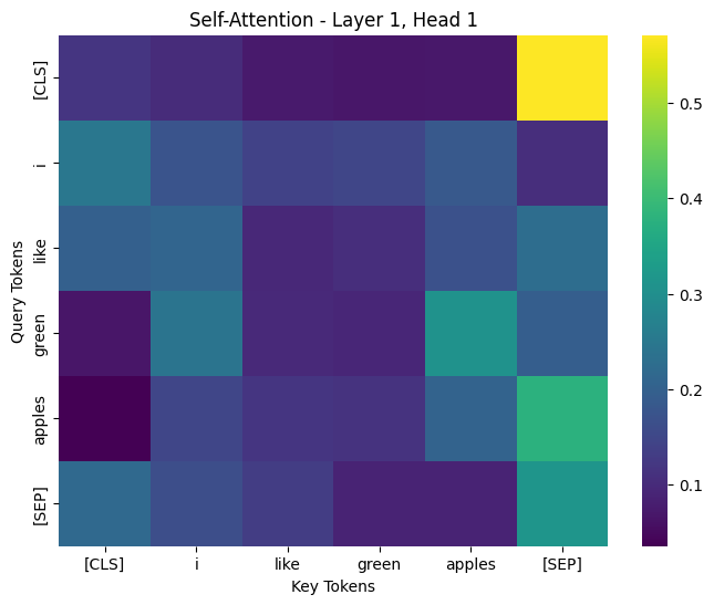
The resulting heatmap gives us a visual representation of the attention matrix.

The heatmap can initially look confusing, so it helps to map the axes directly to the attention equation.

The rows represent query positions. The columns represent key positions.

A brighter cell means that the query token is assigning a larger attention weight to that key token.

For example, we see a bright cell at the intersection of the Apples row and the Green column. This indicates the Apples query is attending strongly to Green in that particular head and layer.

However, one thing to note is that different attention heads can exhibit different patterns.

Some heads may focus heavily on nearby tokens.

Others may produce longer-range patterns.

Some may appear to focus on particular grammatical relationships.

The important point is that the attention matrix is dynamic. It depends on the input sentence.

This is fundamentally different from the fixed averaging matrix we used earlier.

One other thing to note is that while Attention is one of the key components in a Transformer, it’s not a complete explanation of the model.

A Transformer layer also contains:

• residual connections,
• feed-forward / MLP layers,
• normalisation,
• projections,
• interactions across multiple layers,
• and multiple attention heads.

Important model behaviour can emerge from the interaction of all these components.

Therefore, attention maps are best viewed as diagnostic evidence about information flow, rather than a complete explanation of model reasoning.

⋅ • ✦ • ⋅

Putting Everything Together

We can now connect all four stages of the journey.

Stage 1: Tokenization

Text is converted into discrete token IDs.

"I like Green Apples"
        ↓
[token ID, token ID, token ID, ...]

The tokenizer determines the vocabulary and therefore the basic units the model processes.

⋅ • ✦ • ⋅

Stage 2: Embedding

Each token ID is mapped to a learned vector.

Token ID
   ↓
Embedding lookup
   ↓
[0.32, 0.59, ...]

At this stage, the model knows something about the learned representation of each token, but the representation is not yet fully contextual.

⋅ • ✦ • ⋅

Stage 3: Self-Attention

Each token creates Query, Key, and Value representations.

previous embedding, current embedding
     ↓
 Attention
     ↓
Contextual representation
[0.32, 0.59, ...] -> [0.21, -0.73, ...]

The model dynamically determines which other tokens are relevant.

Causal masking prevents a decoder-only language model from looking at future tokens.

⋅ • ✦ • ⋅

Stage 4: Logits and Sampling

After passing through Transformer layers, the model produces logits over the vocabulary. Which are converted into probabilities using softmax. A decoding strategy is then used to select the next token.

The generated token is then appended to the sequence and the process repeats.

Text -> Tokens -> Embeddings -> Contextual Representations -> Logits -> Probabilities -> Next Token